24 Continuous-Time MC

#MarkovChain #TransitionMatrix #CKEquation

1 Definition of CTMC

A continuous-time Markov Chain(CTMC) is ${X_{t}, t \geq 0}$ on finite or countably infinite state space $S$ satisfying $P (X_{t_{n}} = i_{n} | X_{t_{1}} = i_{1}, \dots, X_{t_{n - 1}} = i_{n - 1}) = P (X_{t_{n}} = i_{n} | X_{t_{n - 1}} = i_{n - 1})$ for all times $0 \leq t_{1} < \dots < t_{n}$ and all states $i_{1}, \dots, i_{n} \in S$ .

Compared with DTMC where $t$ is in some sets of integers.

Pasted image 20241218230702.png

Similarly, it is homogeneous if $P (X_{t + n} = j | X_{n} = i) = P (X_{t} = j | X_{0} = i) = p_{i j} (t)$ for all $t, u > 0$ and $i, j \in S$ . $p_{i j} (t)$ here is transition probability, and $P (t) = (p_{i j} (t))_{i, j \in S}$ is transition probability metric.
Since $p_{i j} (0) = δ_{i j}$ , $P (0) = I$ , which is the identity matrix.

Claim (Chapman-Kolmogorov Equation)

For homogeneous MC, $P (t) P (u) = P (t + u), \forall t, u \geq 0.$

Proof

$\forall i, j \in S$ , $\begin{aligned} P_{i j} (t + u) & = P (X_{t + u} = j | X_{0} = i) \\ = \sum_{X \in S} \underset{P (X_{t + u} = j | X_{u} = k) = p_{k j} (u)}{\underset{⏟}{P (X_{t + u} = j | X_{u} = k, X_{0} = i)}} \cdot \underset{p_{i k} (u)}{\underset{⏟}{P (X_{u} = k | X_{0} = i)}} . \end{aligned}$

2 Constraints on CTMC

Standard CTMC

${P (t)}$ is called standard if $lim_{h \to 0^{+}} P (h) = I$ .

Claim (Continuity of CTMC)

${P (t)}$ is standard $\Rightarrow$ $p_{i j} (t)$ is a continuous function of $t$ $\forall i, j \in S$ .

Proof

$\forall t > 0$ , by CK Equation, $\begin{aligned} | p_{i j} (t + h) - p_{i j} (t) | & = | \sum_{k \in S} p_{i k} (h) p_{k j} (t) - p_{i j} (t) | \\ = | (p_{i i} (h) - 1) p_{i j} (t) + \sum_{k \neq i} p_{i k} (h) p_{k j} (t) | \\ \leq (1 - p_{i i} (h)) p_{i j} (t) + \sum_{k \neq i} p_{i k} (h) \\ = (1 - p_{i i} (h)) p_{i j} (t) + (1 - p_{i i} (h)) \to 0, h \to 0^{+}, \end{aligned}$
since $lim_{n \to 0^{+}} p_{i i} (h) = 0$ by condition.

Theorem

Let ${P (t)}$ be standard. Then $\forall i, j \in S$ , the following rates exist:

$q_{i} \overset{Δ}{=} lim_{h \to 0^{+}} \frac{1 - p_{i i} (h)}{h} \in [0, \infty]$ .
$q_{i j} \overset{Δ}{=} lim_{h \to 0^{+}} \frac{p_{i j} (h)}{h} \in [0, \infty]$ .

Constraints on MC

With $q_{i i} = - q_{i}$ , $Q = (q_{i j})_{i, j \in S}$ is called the generator/Q matrix of the Markov Chain.
${X_{t}}$ is called stable if $q_{i} < \infty, \forall i \in S$ .
${X_{t}}$ is called conservative if $q_{i} = \sum_{j \neq i} q_{i j}, \forall i \in S$ .

We will assume standard, stable and conservative MC. Under such case, we can show $p_{i i} (h) = 1 - q_{i} h + o (h), p_{i j} (h) = q_{i j} h + o (h) .$

3 Differentiation of Transition Matrix

Kolmogorov Forward Equation

$\frac{d P (t)}{d t} = P (t) Q .$

Here $\frac{d P (t)}{d t} = lim_{h \to 0^{+}} \frac{P (t + h) - P (h)}{h}$ .

Proof

$\begin{aligned} \frac{d P (t)}{d t} & = lim_{h \to 0^{+}} \frac{P (t + h) - P (h)}{h} = lim_{h \to 0^{+}} \frac{P (t) P (h) - P (t)}{h} \\ = P (t) lim_{h \to 0^{+}} \frac{P (h) - I}{h} = P (t) Q . \end{aligned}$

Similarly

Kolmogorov Backward Equation

$\frac{d P (t)}{d t} = Q P (t) .$

If initial condition is $P (0) = I$ , the unique solution $P (t) = e^{t Q} = \sum_{k = 0}^{\infty} \frac{(t Q)^{k}}{k!} .$

Claim

$\sum_{j \in S} [P (t)]_{i j} = 1, \forall i \in S .$

Proof

Since row sums of $Q$ are all zero, by KFE $\frac{d P (t)}{d t} \cdot \vec{1} = P (t) Q \vec{1} = \vec{0},$ so $P (t) \cdot \vec{1} = \vec{C}$ is a constant vector. Since $P (0) = I$ , $\vec{C} = \vec{1}$ .

Claim (Holding Time)

Suppose $X_{(t)} = i \in S$ . Then $H = inf {u > 0 | X (t + u) \neq i} \sim Exp (q_{i})$ .

Proof

For $a, b > 0$ , $\begin{aligned} P (H > a + b | H > a) & = P (H > a + b | X (t + a) = i) \\ = P (H > b), \end{aligned}$
so $H \sim Exp (λ)$ for some $λ$ .
c.d.f $F_{H} (u) = P (H \leq u) = 1 - e^{- λ u}$ , differentiate it we have $F_{H}^{'} (0) = λ .$
On the other hand $\begin{aligned} 1 - F_{H} (u) = P (H > u) = [P (u)]_{i i} \\ \Rightarrow & F_{H}^{'} (u) = - [P^{'} (u)]_{i i} = - [P (u) Q]_{i i} . \end{aligned}$
Since $P (0) = I$ , by KFE $F_{H}^{'} (0) = - [I Q]_{i i} = - q_{i i} = q_{i} .$

Example 1 (Poisson Process)

${X_{t}}$ on $S = N$ . With $Q = [\begin{matrix} - λ & λ & 0 & 0 & 0 & \dots \\ 0 & - λ & λ & 0 & 0 & \dots \\ 0 & 0 & - λ & λ & 0 & \dots \\ ⋮ & ⋮ & ⋮ & ⋱ & ⋱ & ⋱ \end{matrix}] .$
We want to compute $P (X_{t} = j | X_{0} = 0) = [P (t)]_{0 j}$ . By KFE, $P^{'} (t) = P (t) Q \Rightarrow [P^{'} (t)]_{00} = [P (t)]_{00} q_{00} = - λ [P (t)]_{00},$
since $[P (0)]_{00} = [I]_{00} = 1$ , so $[P (t)]_{00} = e^{- λ t}$ .
For $j \geq 1$ , $[P^{'} (t)]_{0 j} = [P (t)]_{0 j} q_{j j} + [P (t)]_{0, j - 1} q_{j - 1, j},$ so by induction, $[P (t)]_{0 j} = \frac{(λ t)^{j} e^{- λ t}}{j!} .$

Example 2 (Birth Death Processes)

$Q = [\begin{matrix} - λ_{0} & λ_{0} \\ μ_{1} & - (μ_{1} + λ_{1}) & λ_{1} \\ μ_{2} & - (μ_{2} + λ_{2}) & λ_{2} \\ ⋱ & ⋱ & ⋱ \end{matrix}] .$

A system of coupled ODEs from KBE: $\begin{aligned} P_{0 j}^{'} (t) & = - λ_{0} P_{0 j} (t) + λ_{0} P_{1 j} (t), \\ P_{i j}^{'} (t) & = μ_{i} P_{i - 1, j} (t) - (μ_{i} + λ_{i}) P_{i j} (t) + λ_{i} P_{i + 1, j} (t), i \geq 1, \end{aligned}$ boundary condition: $P_{i j} (0) = δ_{i j}$ .

The closed form solutions are known for various special cases.

Otherwise the system can be solved numerically.

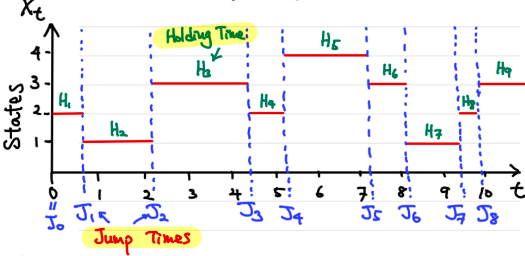
4 Jump Process, Jump Chain, Embedded Chain

For DTMC, ${Y_{n} | n \in N_{0}}$ given by $Y_{n} = X_{J_{n}}$ , where $J_{n}$ is the $n$ th jump time.

Theorem

The transition matrix $\tilde{P} = ({\tilde{p}}_{i j})$ of the embedded jump chain is given by $\begin{aligned} {\tilde{p}}_{i i} & = {\begin{aligned} 0, q_{i i} \neq 0, \\ 1, q_{i i} = 0, \end{aligned} \forall i \in S, \\ {\tilde{p}}_{i j} & = \frac{q_{i j}}{q_{i}} = \frac{q_{i j}}{- q_{i i}}, \forall i, j \in S, i \neq j . \end{aligned}$
Furthermore, $n$ -th holding time $H_{n} ⊥ ⊥ Y_{n}$ .